In 2017, researchers at Google published a paper that proposed a novel neural network architecture for sequence modelling. The paper was called "Attention Is All You Need" by A. Vaswani et al. The name was indeed catchy and so in time to follow there were at least 50 such papers which got published which had a similar ring to its name. The transformer architecture outperformed recurrent neural networks (RNNs), its variations LSTMs and GRUs on machine learning tasks. The AI community embraced it wholeheartedly and wrote several annotated transformer papers and in no time it became a tool for all practitioners and researchers in this field.

Fast forward to 2023, it still is the defacto architecture or a baseline architecture for the deep learning models across natural language processing (NLP) and computer vision (CV). The best-known are the two classes of models, one took the encoder side of the transformer architecture called Bidirectional Encoder Representations from Transformers (BERT) and the other one was built on the decoder side of the transformer architecture called Generative Pretrained Transformers (GPT).

In this blog, I will go over in some detail this famous Transformer architecture and implement a simplistic version of it in PyTorch which will give a nice refresher to our old friend.

I could not be more thankful to the entire AI community for disseminating this valuable knowledge which has shaped innumerable companies, added value to customers all over the globe and given us incessant challenges to solve and shape our professional and personal lives.

My primary source for this blog will be from HuggingFace and would like to thank Lewis Tunstall, Leandro von Werra & Thomas Wolf for writing some excellent and palatable technical blogs on AI.

The Transformer Architecture

The transformer architecture is made up of both the encoder and decoder and that's the reason tasks like Machine Translation are aptly suited for such architecture. In Machine Translation, a text is translated from one language to another. Hence the need for both an encoder and a decoder.

However, it should be known that the transformer architecture is not constrained to similar kinds of tasks. As mentioned above how BERT used the encoder and GPT used the decoder architecture of the transformer. Also, models like BART and T5 used for the encoder and decoder blocks in their architecture

Let's go over the main two components of the transformer architecture -

1. Encoder: This converts an input sequence of tokens into a sequence of embedding vectors. These are also known as context vectors or hidden state vectors.

2. Decoder: It uses the encoder's hidden state to iteratively generate an output sequence of tokens, one token at a time.

Here in the above figure, the top part in blue is the Encoder block and the one in Red is the Decoder block. These are the main things happening inside these blocks -

• The input text which is in English is tokenized and converted to token embeddings using some techniques like Wordpiece or Sentencepiece where words are broken into subwords and they get some numeral numbers including some special tokens denoting the start and other markers.

• To provide the transformer model with the positional information of the tokens we add the positional embeddings with the token embeddings.

• The encoder comprises a stack of encoder blocks through which the input embeddings passed and at the end of the encoder, a rich contextualized hidden state vector is created.

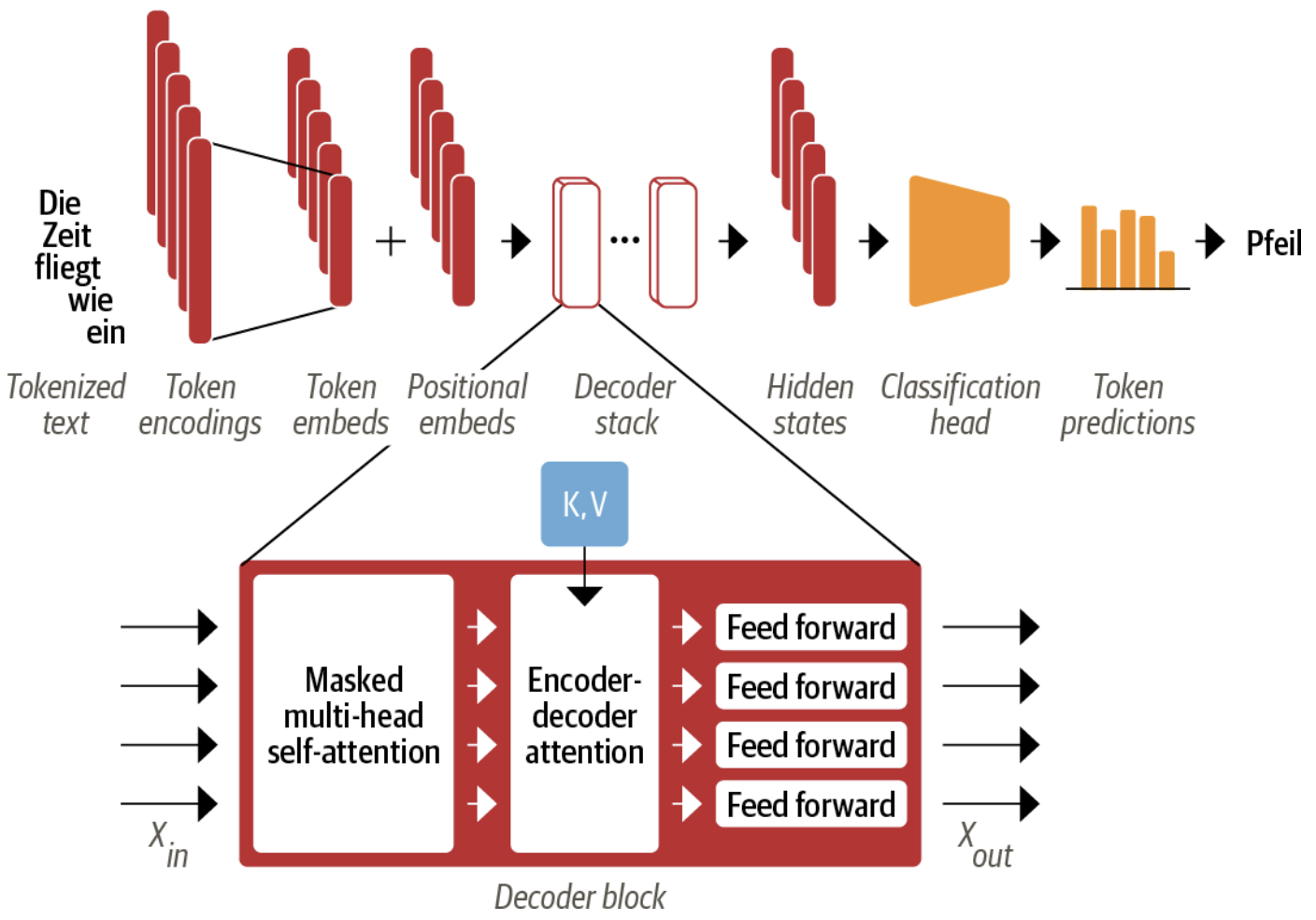
• The encoder's output is fed to each decoder layer, and the decoder then generates, a prediction for the most probable next token in the sequence. The output of this step is then fed back into the decoder to generate the next token, and so on until a special end-of-sequence (EOS) token or the maximum length is reached.

• Here, in the above example, the entire sequence but one is already generated. At this point, the decoder gets the contextualized hidden state vector of the encoder along with the previously generated texts to generate the final token which in this case is "Pfeil" which in German means arrow.

Let's take a deeper dive to understand the inner workings of the encoder and decoder blocks

The Encoder

We have seen that the encoder comprises many encoder layers stacked next to each other. Each encoder layer receives a sequence of embeddings which is further passed through the below sub-layers

• A multi-head self-attention layer

• A fully connected feed-forward layer is applied to each input embedding.

In the above figure, we could see those sub-layers inside the encoder block. Also, the shape of the input and the output is the same i.e. Xin.shape() == Xout.shape() But what changes are the vector representation as in each step along the way the contextualized vector becomes richer i.e. words like "bank" will be updated to be more "financial institution-like" and less "river bank-like" if words like "savings" or "deposits" are close to it.

Each of these sublayers also uses skip connections and layer normalization which are some standard tricks to train deep neural networks effectively.

However, there is one more building block of the transformer called the self-attention layer which makes the transformer architecture so effective.

Self-Attention

Each token in a sequence is mapped to a vector of some fixed dimensions. For example, in BERT each token is mapped to a fixed 768-dimensional vector. "Attention" is a way to assign different weights to each of these elements in a sequence.

The "self" refers to the fact that these weights are computed for all hidden states of the encoder. This is very different from the recurrent models where the attention is calculated between each encoder's hidden state to the decoder's hidden state at the time of decoding.

Instead of using a fixed embedding for each token, the attention mechanism computes a weighted average of each embedding concerning the whole sequence.

To formally define it, given a sequence of token embeddings x1, x2, ....., xn, self-attention produces a sequence of new embeddings x1', x2', ...., xn' where each xi' is a linear combination of all the xj .

$$x_{i}' = \sum_{j=1}^{n} w_{ji}x_{j} \quad \text{such that} \quad \sum_{j}w_{ji} = 1$$

The coefficients wji are called attention weights and are normalized. Taking a weighted average and keep taking it for all the encoder blocks will create rich contextualized embeddings for a token related to all the other tokens.

So, now the question is how do we calculate these attention weights which are denoted by wji The technique used in the paper is by taking the scaled dot-product attention and this is how it works -

• Project each token embedding into three vectors called query, key, and value.

• Determine how much the query and key vectors relate to each other using a similarity function, in this case, it is the dot product. The queries and the keys that are similar will have large dot product and vice versa. So for a sequence of 'n' tokens, there will be n x n matrix of Attention Scores.

• The attention scores are normalized by multiplying by a scaling factor and then passing it through the softmax to ensure that all column values sum to 1. The resulting n x n matrix is now the Attention Weights.

• The attention weights are multiplied by the value vector v1, v2,...vn to obtain the updated representation for the embedding denoted in the above equation.

Implementation using PyTorch

Before we implement the blocks let's take a look at the self-attention weights for the below text -

"After his meeting in the bank he came back home, and took a leisure walk along the bank of the river which flows through his town"

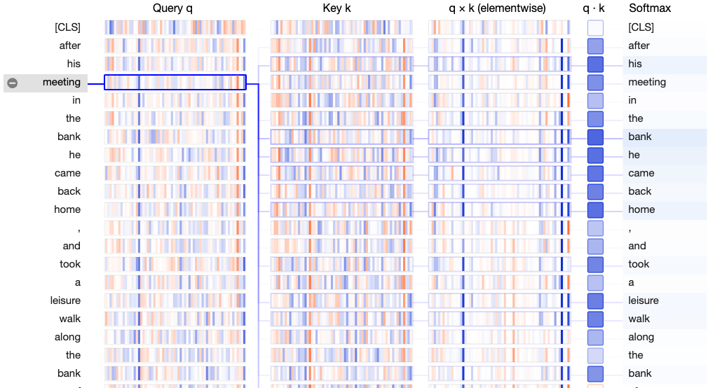
We can see that the query vector "meeting" is contextually more associated with the words "bank he came back home".

To implement the self-attention we will build this workflow. You can also follow this Colab Notebook.

Tokenize the text

from transformers import AutoTokenizer
model_ckpt = "bert-base-uncased"
tokenizer = AutoTokenizer.from_pretrained(model_ckpt)
model = BertModel.from_pretrained(model_ckpt)

Each token in the above sentence has been mapped to a unique ID in the tokenizer's vocabulary -

inputs = tokenizer(text, return_tensors = "pt", add_special_tokens = False)

print(inputs.input_ids)

tensor([[ 2044,  2010,  3116,  1999,  1996,  2924,  2002,  2234,  2067,  2188, 1010,  1998,  2165,  1037, 12257,  3328,  2247,  1996,  2924,  1997, 1996,  2314,  2029,  6223,  2083,  2010,  2237]])

Create dense embeddings

from torch import nn 
from transformers import AutoConfig

config = AutoConfig.from_pretrained(model_ckpt)
token_emb = nn.Embedding(config.vocab_size, config.hidden_size)
print(token_emb)

#Embedding(30522, 768)

inputs_embeds = token_emb(inputs.input_ids)
inputs_embeds.size()

# torch.Size([1, 27, 768]) i.e. [batch_size, seq_len, hidden_dim]

These token embeddings are independent of the context. This means homonyms (words with the same spelling but different meanings) has the same vector representation. In the above representation, the word "bank" has 2924 value for both contexts.

Self Attention

Create query, key and value vectors and calculate attention scores using the dot product as the similarity function.

import torch
from math import sqrt
import torch.nn.functional as F

def scaled_dot_product_attention(query, key, value):
 dim_k = query.size(-1)
 scores = torch.bmm(query, key.transpose(1, 2)) / sqrt(dim_k)
 # scores : torch.Size([1, 27, 27])
 weights = F.softmax(scores, dim=-1)
 return torch.bmm(weights, value)  # torch.Size([1, 27, 768])

torch.bmm() calculates the dot product between two matrices in the batch independently. We further scale it using softmax and multiply the attention weights by the values.

Multi-headed attention

Here the vectors Q, K, and V have multiple sets of linear projections where each one represents an attention head. The total is called multi-headed attention. This ensures that each softmax from an attention head focuses on one specific aspect of the similarity. One could be subject-verb agreement, another one could be the presence of qualifiers, quantifiers etc. That's the reason the initial projection is randomly distributed and they are learnable.

class AttentionHead(nn.Module):
  def __init__(self, embed_dim, head_dim):
    super().__init__()
    self.q = nn.Linear(embed_dim, head_dim)
    self.k = nn.Linear(embed_dim, head_dim)
    self.v = nn.Linear(embed_dim, head_dim)

  def forward(self, hidden_state):
    attn_outputs = scaled_dot_product_attention(
        self.q(hidden_state), self.k(hidden_state), self.v(hidden_state))
    return attn_outputs

class MultiHeadAttention(nn.Module):
  def __init__(self, config):
    super().__init__()
    embed_dim = config.hidden_size
    num_heads = config.num_attention_heads
    head_dim = embed_dim // num_heads
    self.heads = nn.ModuleList(
        [AttentionHead(embed_dim, head_dim) for _ in range(num_heads)]
    )
    self.output_linear = nn.Linear(embed_dim, embed_dim)

  def forward(self, hidden_state):
    x = torch.cat([h(hidden_state) for h in self.heads], dim = -1)
    x = self.output_linear(x)
    return x

Hare, head_dim is the number of dimensions we are projecting into. For example, BERT has 12 attention heads, so the dimension of each head is 768 / 12 = 64. The multi-attention head is the concatenation of the outputs from the single-attention head.

The Feed-Forward Layer

This is the sub-layer in the both encoder and decoder block. It is a two-layer fully connected neural network.

class FeedForward(nn.Module):
  def __init__(self, config):
    super().__init__()
    self.linear_1 = nn.Linear(config.hidden_size, config.intermediate_size)
    self.linear_2 = nn.Linear(config.intermediate_size, config.hidden_size)
    self.gelu = nn.GELU()
    self.dropout = nn.Dropout(config.hidden_dropout_prob)

  def forward(self, x):
    x = self.linear_1(x)
    x = self.gelu(x)
    x = self.linear_2(x)
    x = self.dropout(x)
    return x

Layer Normalization & Skip Connections

• Layer Normalization: It normalizes each input in the batch to have zero mean and unity variance.

• Skip Connections: They pass a tensor to the next layer of the model without processing and add it to the processed tensor.

Layer normalization can have two choices -

• Post-layer normalization: The transformer paper places post-layer normalization between the skip connections. While training in this setup from scratch the gradients can diverge, hence there is a hyperparameter called learning rate warm-up is used. Here, the learning is gradually increased from a small value to some maximum value during training.

• Pre-layer normalization: It places layer normalization within the span of the skip connections. This is much more stable and does not require a learning rate warmup.

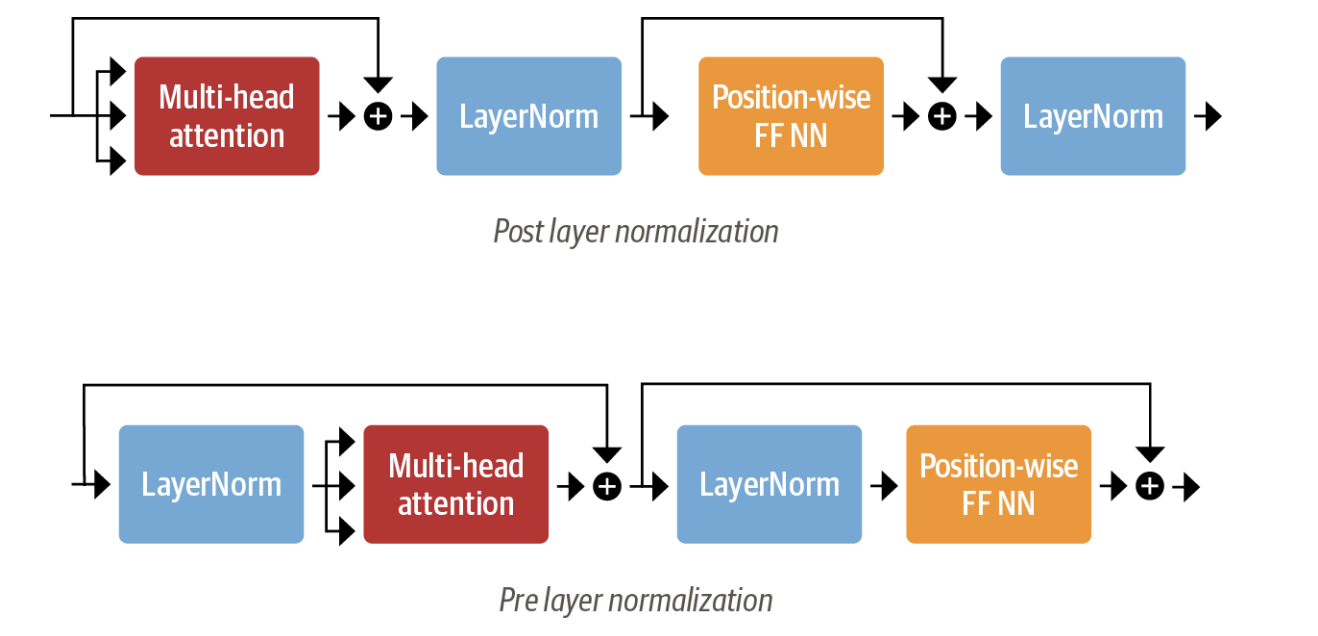
We will be using the pre-layer normalization.

class TransformerEncoderLayer(nn.Module):
  def __init__(self, config):
    super().__init__()
    self.layer_norm_1 = nn.LayerNorm(config.hidden_size)
    self.layer_norm_2 = nn.LayerNorm(config.hidden_size)
    self.attention = MultiHeadAttention(config)
    self.feed_forward = FeedForward(config)

  def forward(self, x):
    # pre-layer norm
    hidden_state = self.layer_norm_1(x)
    # attention with skip connection
    x = x + self.attention(hidden_state)
    x = x + feed_forward(self.layer_norm_2(x))
    return x

Positional Embeddings

Augment the token embeddings with a position-dependent pattern of values arranged in a vector. Here we will create a custom Embeddings module that combines a token embedding layer that projects the input_ids to a dense hidden state together with the positional embedding that does the same for position_ids. The resulting embedding is the sum of both embeddings.

class Embeddings(nn.Module):
  def __init__(self, config):
    super().__init__()
    self.token_embeddings = nn.Embedding(config.vocab_size,
                                         config.hidden_size)
    self.position_embeddings = nn.Embedding(config.max_position_embeddings,
                                             config.hidden_size)
    self.layer_norm = nn.LayerNorm(config.hidden_size, eps = 1e-12)
    self.dropout = nn.Dropout()

  def forward(self, input_ids):
    # create position IDs for input sequence
    seq_length = input_ids.size(1)
    position_ids = torch.arange(seq_length, dtype = torch.long).unsqueeze(0)

    # create token and position embeddings
    token_embeddings = self.token_embeddings(input_ids)
    position_embeddings = self.position_embeddings(position_ids)

    # combine token and position embeddings
    embeddings = token_embeddings + position_embeddings
    embeddings = self.layer_norm(embeddings)
    embeddings = self.dropout(embeddings)
    return embeddings

Transformer Encoder

Using the above classes and combining the embeddings with the encoder layers we get the final transformer encoder. Here it is -

class TransformerEncoder(nn.Module):
  def __init__(self, config):
    super().__init__()
    self.embeddings = Embeddings(config)
    self.layers = nn.ModuleList([TransformerEncoderLayer(config) for _ in range(config.num_hidden_layers)])

  def forward(self, x):
    x = self.embeddings(x)
    for layer in self.layers:
      x = layer(x)
    return x

# Let's check the output of the encoder -

encoder = TransformerEncoder(config)
encoder(inputs.input_ids).size()

# torch.Size([1, 27, 768])

The output returns a hidden state for each token in the batch.

Classification Head

The above implementation is also called a task-independent body. If we want to do a classification task, we would add a classification head to the body.

The output of the encoder body returns a hidden state for each token. But for the classification task, we just need one such token. In practice, we use the first token also known as [CLS] token. Further on we add a dropout layer with a linear layer to make the classification prediction.

class TransformerForSequenceClassification(nn.Module):
  def __init__(self, config):
    super().__init__()
    self.encoder = TransformerEncoder(config)
    self.dropout = nn.Dropout(config.hidden_dropout_prob)
    self.classifier = nn.Linear(config.hidden_size, config.num_labels)

  def forward(self, x):
    # select the hidden state of [CLS] token
    x = self.encoder(x)[:, 0, :]
    x = self.dropout(x)
    x = self.classifier(x)
    return x

config.num_labels = 3
encoder_classifier = TransformerForSequenceClassification(config)
encoder_classifier(inputs.input_ids).size()

# torch.Size([1, 3])

The output is for each example in the batch we get the unnormalized logits for each class in the output.

The Decoder

We will not implement the decoder as a lot of building blocks could be reused. But we will go over the architecture and recognize the difference.

The difference in the decoder layer are as follows -

• Masked multi-head self-attention layer: This ensures that the tokens generated at each timestep are only based on the past outputs and the current token being predicted.

• Encoder-decoder attention layer: Performs multi-head attention over the output key and the value vectors of the encoder stack with the intermediate representations of the decoder acting as the queries. This way the encoder-decoder attention layer learns how to relate tokens from two different sequences, such as two different languages. The decoder has access to the encoder keys and values in each block.

Colab Notebook

Paper: Attention is All You Need

Code: Colab Notebook

Author's Note

In this blog, we reviewed the inner workings of the famous Transformer architecture. In several ways this learning could be useful -

• How the self-attention mechanism works which is fundamental to the transformer model and its efficacy

• How to represent system architecture in modular classes.

• A good refresher to PyTorch modules.

• Nonetheless, this hands-on implementation makes things more visible and could be extended to various applied works in Deep Learning.

Thank you ...

I also love solving problems related to NLP and Deep Learning. If you wish to collaborate please reach out to me through my LinkedIn profile. Will be happy to connect.